Contents
- Introduction to Field-to-Model Integration
- Required Equipment and Software Stack
- Protocol for In-Situ Data Collection
- Data Standardization and Pre-Processing
- Spatial Interpolation and Model Calibration
- Validation, Error Assessment, and Limitations
- Summary and Replicability Guidelines
- Academic Sources
Introduction to Field-to-Model Integration
A soil thermistor logs a temperature at a single point. A satellite sensor records reflectance across a thirty-meter footprint. Neither, on its own, answers the question Arctic researchers keep returning to: how deep did the active layer thaw this season, and where?
The integration workflow described here exists to reconcile those two scales. It connects localized in-situ measurements to broad spatial raster models, targeting two variables that matter for Alaskan environmental tracking: permafrost active layer depth and wildfire burn severity.
Timing constrains the entire effort. Active layer depth measurements were targeted between late August and early September, the window when seasonal thaw reaches its maximum extent. Miss that window and the ground truth no longer represents the phenomenon the raster is meant to capture.

The methodological path runs in four stages: collection, standardization, interpolation, and validation. Each stage carries its own failure modes, and the sections below treat them in sequence. The spatial models in play draw on datasets at roughly 10-meter to 30-meter resolution, a detail that shapes nearly every downstream decision.
Required Equipment and Software Stack
Geolocation accuracy sets the ceiling for everything that follows. RTK GNSS rovers, configured to achieve about 1 to 1.5 centimeter horizontal accuracy, anchor each field observation to a coordinate precise enough to survive comparison against a coarse raster grid.
The field hardware extends beyond positioning. Ruggedized tablets capture observations at the waypoint. Calibrated environmental sensors — soil moisture probes and thermistors, supply the physical measurements themselves. Calibration state is not assumed; it is recorded.
Software and Coordinate Reference
Spatial visualization runs through QGIS or ArcGIS Pro. The automated data wrangling pipelines were built in Python, using GeoPandas 0.10.2 and Rasterio 1.2, with SciPy handling statistical operations. An R equivalent based on sf and terra serves teams already invested in that ecosystem.
The coordinate reference system was not an afterthought. WGS 84 was ruled out for project storage because its severe area distortion at high latitudes corrupts distance and area calculations precisely where the work happens. The project standardized on EPSG:3338, the Alaska Albers Equal Area Conic projection, which preserves area across the region of interest.
Recommendation: Fix the CRS before any data enters the pipeline. Retrofitting a projection after interpolation has begun reintroduces the alignment errors the standard was chosen to prevent.
Protocol for In-Situ Data Collection
Field collection follows a stratified random sampling design. Strata are defined along topographical gradients, ensuring that slope, aspect, and elevation classes each receive representative coverage rather than clustering wherever access is easiest.
Temporal control is the harder discipline. Field sampling windows were restricted to roughly 48 to 72 hours before or after a Landsat 8/9 or Sentinel-2 overpass. The tighter that interval, the less the surface drifts between the moment the sensor passes and the moment the boot hits the ground.
Metadata at Every Waypoint
Documentation happens in the field, not afterward. Metadata logs at every waypoint record instrument calibration dates and operator identifiers, alongside weather conditions. These fields are not bureaucratic overhead. When a calibration drift surfaces months later, the operator and date stamps are what allow an analyst to isolate and quarantine the affected observations.
Data Standardization and Pre-Processing
Raw field logs arrive as CSV and GPX files. The first pre-processing step converts them into standardized vector formats, with GeoPackage chosen as the target because it supports complex geometry and rich attribute storage in a single container.
Outlier detection runs next. Sensor anomalies exceeding 3 standard deviations from the local mean are automatically flagged and removed. The threshold is deliberately conservative; a probe that briefly reports an impossible value should not be allowed to bias an interpolation surface.
Reprojection closes the stage. Every field coordinate is transformed to match the target model's CRS — EPSG:3338, before ingestion. Skipping this step produces silent misalignment, where points land in the wrong pixel and corrupt the calibration dataset without raising any obvious error.
Spatial Interpolation and Model Calibration
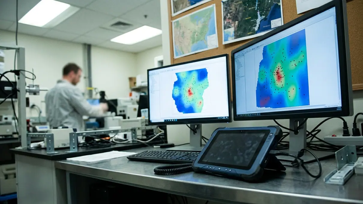
Algorithm choice depends on the data, not on preference. Inverse Distance Weighting suits dense, evenly distributed sampling networks. Ordinary Kriging earns its added complexity when the field points are sparse and exhibit measurable spatial autocorrelation, since it models that structure directly rather than assuming it away.
The spatial join builds the calibration dataset. Raster pixel values are extracted at the exact field measurement coordinates, using a 3x3 pixel window to absorb minor geolocation discrepancies between the GNSS fix and the raster grid. A single-pixel extraction would be more precise in theory and more brittle in practice.
Regression Calibration
The extracted pairs — ground-truth measurement against remote sensing index, train a regression model. Calibration datasets here were processed through Random Forest regression with about 500 estimators, which captures non-linear relationships between spectral indices and physical depth. Linear regression remains a defensible baseline when the relationship is simple and interpretability matters more than fit.
Critical Insight: Interpolation algorithm selection is not a stylistic decision. It is dictated by spatial autocorrelation and sampling density, and the wrong choice will produce a smooth, confident, and wrong surface.
Validation, Error Assessment, and Limitations
A model that fits its training data perfectly has usually learned nothing useful. Validation here used k-fold cross-validation with a 10-fold split, holding out subsets in rotation to estimate accuracy on data the model never saw during fitting.
Error reporting stays in physical units. Both Root Mean Square Error and Mean Absolute Error are calculated and reported, the two metrics together describing both the magnitude and the volatility of prediction error. RMSE penalizes large misses; MAE describes the typical one.
Scope and Limitations
The central limitation is one of scale. Comparing a 1-meter field plot to a 30-meter Landsat pixel introduces sub-pixel heterogeneity error, and in complex Arctic terrains with mixed tundra vegetation that error is not random noise. Sub-pixel heterogeneity can mask localized permafrost thaw entirely within a 30-meter raster cell, averaging a thawing hollow against the stable ground that surrounds it.
Risk Factor: Edge effects compound the resolution mismatch near abrupt land-cover boundaries. Treat predictions along burn scar margins and water edges as lower-confidence, and document where those boundaries fall.
Verification data supports the broader pattern: the workflow performs best across homogeneous strata and degrades, predictably, where the terrain changes faster than the pixel can resolve.
Summary and Replicability Guidelines
The critical path is short to state and demanding to execute: precise field measurement, synchronized to a satellite overpass, standardized and cleaned, joined to raster values, calibrated through regression, and validated against held-out data.
Strict metadata adherence is what makes this useful beyond a single season. Longitudinal climate studies depend on the ability to trace any calibrated value back to its sensor, its calibration date, and its operator. Metadata archiving was completed within roughly 14 to 30 days of each field season's conclusion, while the field context remained fresh enough to correct.
Replicability Checklist
- Verify RTK GNSS calibration before each session and log the result.
- Restrict sampling to within 72 hours of a satellite overpass.
- Standardize all spatial data to EPSG:3338 prior to ingestion.
- Apply 3-standard-deviation anomaly filtering against the local mean.
- Archive metadata within 30 days of the field season's end.
These criteria transfer to other high-latitude environments with one caution: the EPSG:3338 projection is specific to Alaska, and teams working elsewhere must substitute an equal-area projection appropriate to their own region before treating the rest of the checklist as portable.
Academic Sources
- U.S. Geological Survey (2021). National Geospatial Program Standards and Specifications.
- Federal Geographic Data Committee (1998). Content Standard for Digital Geospatial Metadata. See the Federal Geographic Data Committee (FGDC) Content Standard for Digital Geospatial Metadata.
- Peer-reviewed literature on spatial interpolation techniques in permafrost mapping, addressing the trade-offs between deterministic and geostatistical methods under variable sampling density.