Why Tundra Fire Maps Matter to Alaska
A perimeter drawn too late can leave an Alaskan community planning around a fire that has already crossed the terrain. A perimeter drawn too broadly can distort estimates of burned vegetation and the climate impacts that follow. Accurate tundra wildfire data matters to people making decisions about subsistence and access, as well as to researchers modeling Arctic change.
Historical Alaska fire records emphasize the boreal forest, where large burns have long shaped expectations about fire behavior. Increasing tundra fire activity calls for a closer look north of that familiar frame. The analysis described here combines MODIS and VIIRS satellite detections across the Brooks Range and North Slope, with a record spanning May 2001 through September 2022. Its purpose is to track changing occurrence and extent through time rather than assign today’s risk from a fixed historical average.
Those two measures answer different questions. An active-fire detection helps locate burning at a particular time. A mapped perimeter shows the area assessed as burned after analysts reconcile imagery and boundary evidence. Keeping them separate is the first safeguard against overstating either fire frequency or fire size.
Finding a Sustained Ignition in Satellite Detections
A cluster of thermal detections can reflect one continuing fire rather than several new ignitions. The occurrence analysis therefore calibrated thermal-anomaly detections to isolate events lasting longer than 48 hours and paired them with ground-truthed ignition coordinates. It examined early-season activity between late May and mid-June, when the timing of new fires can be obscured if analysts compare only whole-season totals.
Separate the Fire Signal From the Season
A practical occurrence workflow starts by grouping detections into candidate events, then checks their locations against verified ignition coordinates. Next, it compares the timing and distribution of those events across seasons. A sustained shift would need to appear across comparable periods and places; one active spring alone would not establish a new fire regime. This approach gives spatial context to the qualitative evidence of more frequent tundra burning without claiming a numerical rate that the supplied record does not report.
Normalized burn ratio, or NBR, can help describe vegetation change after a fire. The mapping protocol excluded NBR thresholds as a standalone measure of high-Arctic thermal anomalies: a change in surface reflectance does not, by itself, establish when a fire ignited. Thermal detections paired with ground coordinates serve the occurrence question more directly.
Detection Gap: Cloud cover and satellite pass frequency can leave 12- to 24-hour gaps on an average day in real-time high-Arctic telemetry. An apparent first detection may therefore follow the actual ignition. That timing uncertainty belongs in any comparison of early-season fires, particularly where response and travel decisions depend on a current map.
Where Brooks Range Burns Grow Larger
Fire size needs a boundary, not a count of hot pixels. The extent analysis uses polygon-based perimeter mapping with 30-meter Landsat 8 imagery with standard settings, examining perimeter expansion during the peak fire seasons of 2015 through 2019. Analysts can compare mapped polygons across available images to distinguish a burn that remains local from one that spreads across a wider region.
Regional segmentation matters here. The protocol treats tundra ecoregions separately, allowing expanding Brooks Range perimeters to be examined alongside the more localized burns identified in the Yukon-Kuskokwim Delta. A statewide average would flatten that difference. It could also invite a misleading inference that every tundra type is experiencing the same change in fire size.
Use the Boundary That Fits the Question
For near-real-time awareness, MODIS and VIIRS detections help identify active burning while a perimeter is still developing. For an assessment of burned area, Landsat-based polygons provide a finer spatial boundary. The first approach wins when speed matters to people following an active fire; the second wins when researchers need to compare burn extent across regions or seasons.
A polygon remains an interpretation of imagery. Analysts should inspect edges where unburned patches, smoke or differing image dates complicate the boundary, then retain the source date and mapping method with the feature. That record lets a later user see whether an apparent expansion represents newly burned ground or a revised outline.
Reading Tundra Fire Alongside Permafrost Change
The boundary between boreal and Arctic fire regimes is useful for organizing research, but it cannot explain an individual burn on its own. A tundra perimeter becomes more informative when researchers place it over permafrost degradation maps and examine what changes inside and around the burned area.
In the described analysis, active-layer thickness measurements were overlaid with post-fire vegetation indices to follow shrubification in previously burned tundra. Post-fire thaw depth was monitored over a 36- to 60-month recovery window. Together, these layers help researchers ask whether a mapped fire overlaps deeper seasonal thaw and a change in vegetation cover. They also provide a way to compare nearby burned and unburned ground without treating a perimeter as a complete measure of ecosystem response.
That comparison has practical consequences. Vegetation transitions can change the conditions represented in future fuel maps, while thaw and altered ground cover can affect routes used for subsistence and access. The spatial overlap identifies places worth closer examination; it does not, by itself, prove that fire caused every measured change. Researchers need the timing of observations and the condition of surrounding terrain to interpret the relationship.
Across Alaska, this layered view connects changing fire patterns with broader environmental change while preserving local distinctions. The question for a North Slope community following a recent burn may be whether a familiar route crosses changing ground. For a climate modeler, it may be how much of the mapped burn intersects terrain vulnerable to thaw. Both questions require a perimeter that can be traced back to its imagery.
Build Fire Forecasts Around Current Conditions
A historical fire return interval summarizes a past pattern. It cannot update itself when daily weather, fuel moisture and the location of new ignitions change. The modeling comparison described in the research facts set dynamic, high-resolution spatial frameworks against legacy static datasets for recent tundra fire risk. Its stated recommendation favors models that ingest daily meteorological variables and real-time fuel-moisture indices.
For a usable mapping workflow, that choice has several concrete steps:
- Maintain georeferenced ignition records and dated satellite detections so analysts can revisit how an event was identified.
- Update tundra ecoregion layers and mapped perimeters as imagery permits, preserving earlier versions rather than silently replacing them.
- Feed current weather and fuel-moisture information into spatial forecasts, then examine risk by region and by the access routes communities use.
- Check forecasts against subsequent detections and revised perimeters before carrying assumptions into the next season.
The supplied modeling work includes simulations for the 2025 through 2030 fire seasons, but it provides no forecast scores or comparative accuracy figures. The case for dynamic modeling rests here on its ability to incorporate changing conditions and test forecasts against observed events, not on an unstated numerical performance claim.